Predicting the price of Airbnb listings is a pretty standard project for most people in the stats / data science / ML space. I mean, the data is fairly comprehensive and large and is easily publicly accessible. So what makes this project any different?

I wanted to try looking at this pretty standard problem through a completely different lens. After taking STATS C173/273 at UCLA (one class btw it’s just cross-listed so the designation is odd) I learned about kriging and spatial prediction and testing techniques. Specifically, accounting for spatial autocorrelation in a variable for predicting new values of the same value.

Generally, this is applied to more natural phenomena, like weather events, that are easily designated as geostatistical events. However, I thought it would make sense to consider Airbnb listing themselves a form of geostatistical data. After all, prices vary by neighborhood and location is a prime determinant of listing price. With that in mind, I decided to see for myself if this was a valid way of price prediction.

Note: All the data used in this report is from the 14 December 2024 report of Airbnb data from https://insideairbnb.com/get-the-data/.

Before I began my actual code, I wanted to set up my R environment to make it a bit more efficient.

library(doParallel)

Loading required package: foreach

Loading required package: iterators

Loading required package: parallel

ncores <- detectCores()
clus <- makeCluster(ncores - 1)
registerDoParallel(clus)

I then loaded in the libraries I planned to use for this project.

library(tidyverse)

── Attaching core tidyverse packages ──────────────────────── tidyverse 2.0.0 ──
✔ dplyr     1.1.4     ✔ readr     2.1.5
✔ forcats   1.0.0     ✔ stringr   1.5.1
✔ ggplot2   3.5.1     ✔ tibble    3.2.1
✔ lubridate 1.9.4     ✔ tidyr     1.3.1
✔ purrr     1.0.4     
── Conflicts ────────────────────────────────────────── tidyverse_conflicts() ──
✖ purrr::accumulate() masks foreach::accumulate()
✖ dplyr::filter()     masks stats::filter()
✖ dplyr::lag()        masks stats::lag()
✖ purrr::when()       masks foreach::when()
ℹ Use the conflicted package (<http://conflicted.r-lib.org/>) to force all conflicts to become errors

library(maps)


Attaching package: 'maps'

The following object is masked from 'package:purrr':

    map

library(geoR)

--------------------------------------------------------------
 Analysis of Geostatistical Data
 For an Introduction to geoR go to http://www.leg.ufpr.br/geoR
 geoR version 1.9-4 (built on 2024-02-14) is now loaded
--------------------------------------------------------------

library(gstat)
library(sf)

Linking to GEOS 3.12.2, GDAL 3.9.3, PROJ 9.4.1; sf_use_s2() is TRUE

library(gridExtra)


Attaching package: 'gridExtra'

The following object is masked from 'package:dplyr':

    combine

library(kableExtra)


Attaching package: 'kableExtra'

The following object is masked from 'package:dplyr':

    group_rows

Before I started working with the data set, I had to do some modification. I selected the predictors I wanted to consider and made sure that no two listings had the same combination of latitude and longitude. I then dropped any observations with NA values and randomly sampled 1000 observations to create the final data set. After this, I created factors for the appropriate values and fixed some issues via manual inspection.

set.seed(0)

austin_listings <- austin_listings_orig %>%
  select(c(longitude, latitude, property_type, room_type, bathrooms, bedrooms, beds, price)) %>%
  distinct(longitude, latitude, .keep_all = TRUE) %>%
  drop_na() %>%
  sample_n(1000) %>%
  mutate_if(is.character, as.factor)
austin_listings$price <- as.numeric(gsub("[^0-9\\.]", "", austin_listings$price))

Data Exploration and non-spatial analysis

Before delving into the analysis, I wanted to do some exploratory data analysis of our finalized dataset.

Data overview

library(DataExplorer)
plot_intro(austin_listings)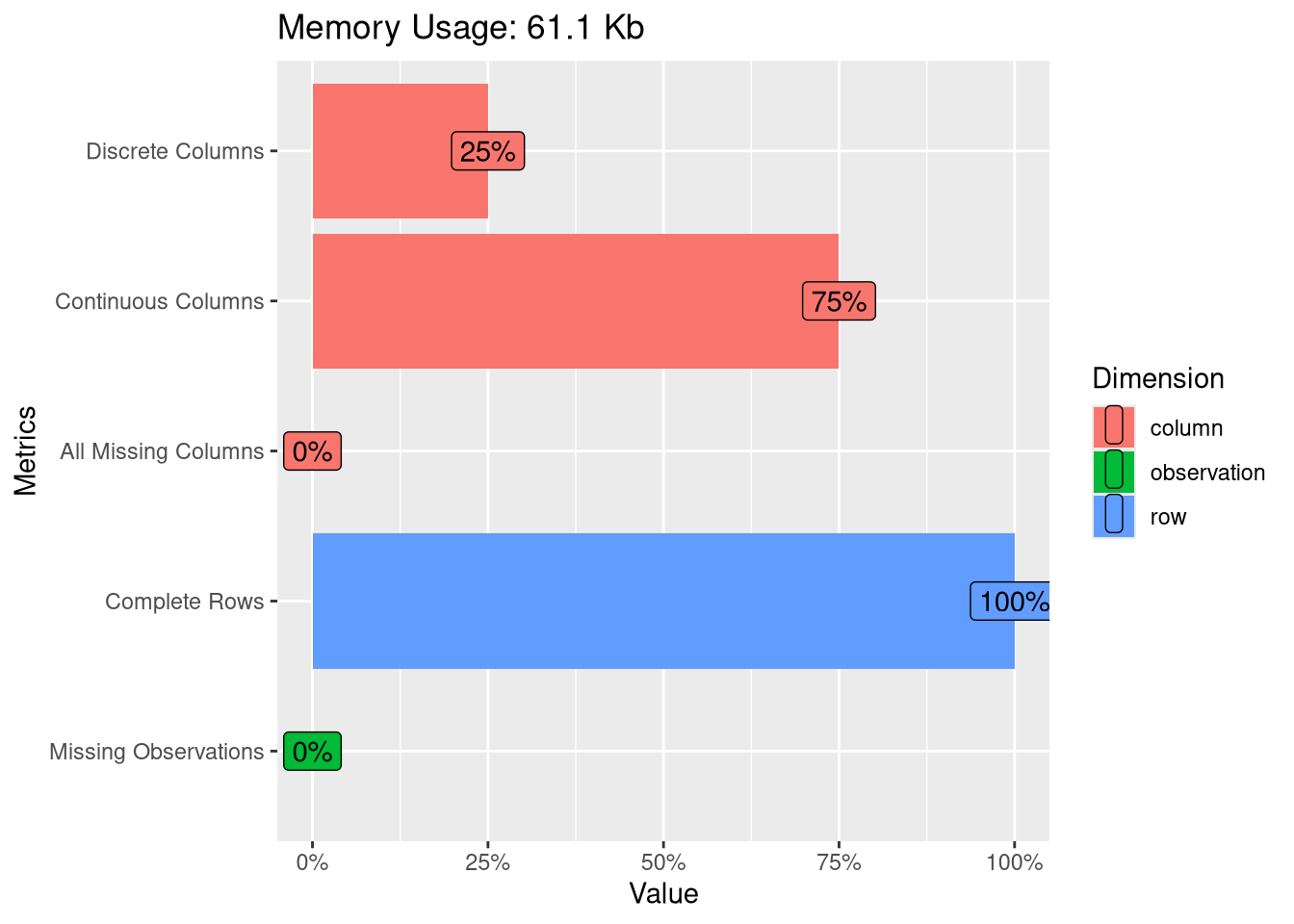

kable(summary(austin_listings))

longitude	latitude	property_type	room_type	bathrooms	bedrooms	beds	price
Min. :-98.01	Min. :30.12	Entire home :430	Entire home/apt:861	Min. :0.000	Min. :0.000	Min. : 0.000	Min. : 18.0
1st Qu.:-97.77	1st Qu.:30.24	Entire rental unit :185	Hotel room : 1	1st Qu.:1.000	1st Qu.:1.000	1st Qu.: 1.000	1st Qu.: 84.0
Median :-97.74	Median :30.27	Private room in home: 94	Private room :135	Median :1.500	Median :2.000	Median : 2.000	Median : 133.0
Mean :-97.75	Mean :30.28	Entire condo : 73	Shared room : 3	Mean :1.698	Mean :2.079	Mean : 2.897	Mean : 256.9
3rd Qu.:-97.72	3rd Qu.:30.31	Entire guesthouse : 62	NA	3rd Qu.:2.000	3rd Qu.:3.000	3rd Qu.: 4.000	3rd Qu.: 225.0
Max. :-97.56	Max. :30.51	Entire guest suite : 22	NA	Max. :7.000	Max. :8.000	Max. :20.000	Max. :10000.0
NA	NA	(Other) :134	NA	NA	NA	NA	NA

Numerical exploration

long_hist <- austin_listings %>% ggplot(aes(x = longitude)) +
  geom_histogram(aes(y = ..density..)) +
  geom_density(col = "red")
lat_hist <- austin_listings %>% ggplot(aes(x = latitude)) +
  geom_histogram(aes(y = ..density..)) +
  geom_density(col = "red")
bed_hist <- austin_listings %>% ggplot(aes(x = bedrooms)) +
  geom_histogram(aes(y = ..density..)) +
  geom_density(col = "red")
bath_hist <- austin_listings %>% ggplot(aes(x = bathrooms)) +
  geom_histogram(aes(y = ..density..)) +
  geom_density(col = "red")
beds_hist <- austin_listings %>% ggplot(aes(x = beds)) +
  geom_histogram(aes(y = ..density..)) +
  geom_density(col = "red")
price_hist <- austin_listings %>% ggplot(aes(x = price)) +
  geom_histogram(aes(y = ..density..)) +
  geom_density(col = "red")

grid.arrange(long_hist, lat_hist, bed_hist, bath_hist, beds_hist, price_hist, nrow = 3)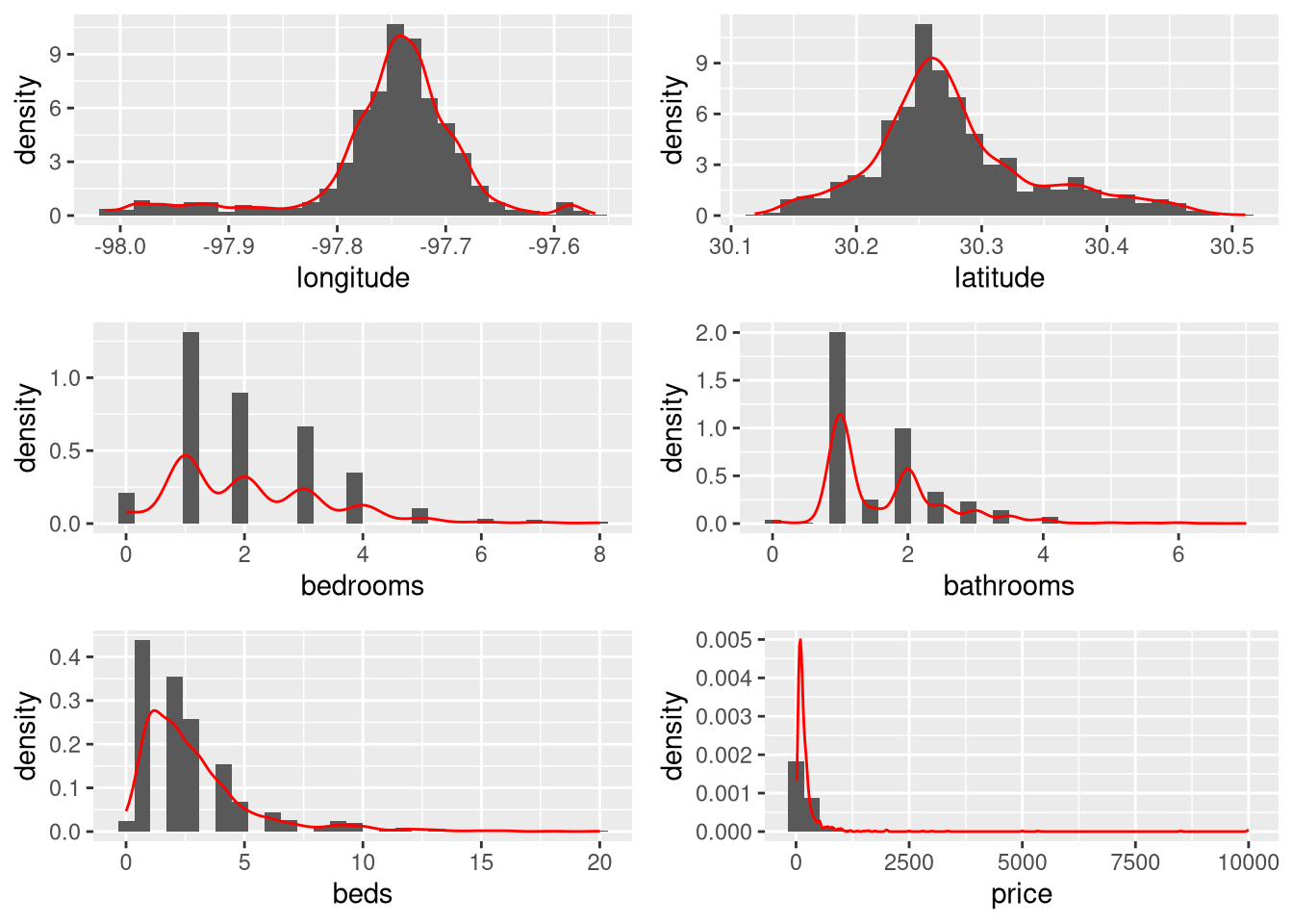

We can see that most of the numeric variables have very skewed distributions.

Categorical data exploration

bar_prop <- austin_listings %>% ggplot(aes(x = property_type)) +
  geom_bar() +
  coord_flip()
bar_room <- austin_listings %>% ggplot(aes(x = room_type)) +
  geom_bar() +
  coord_flip()
grid.arrange(bar_prop, bar_room)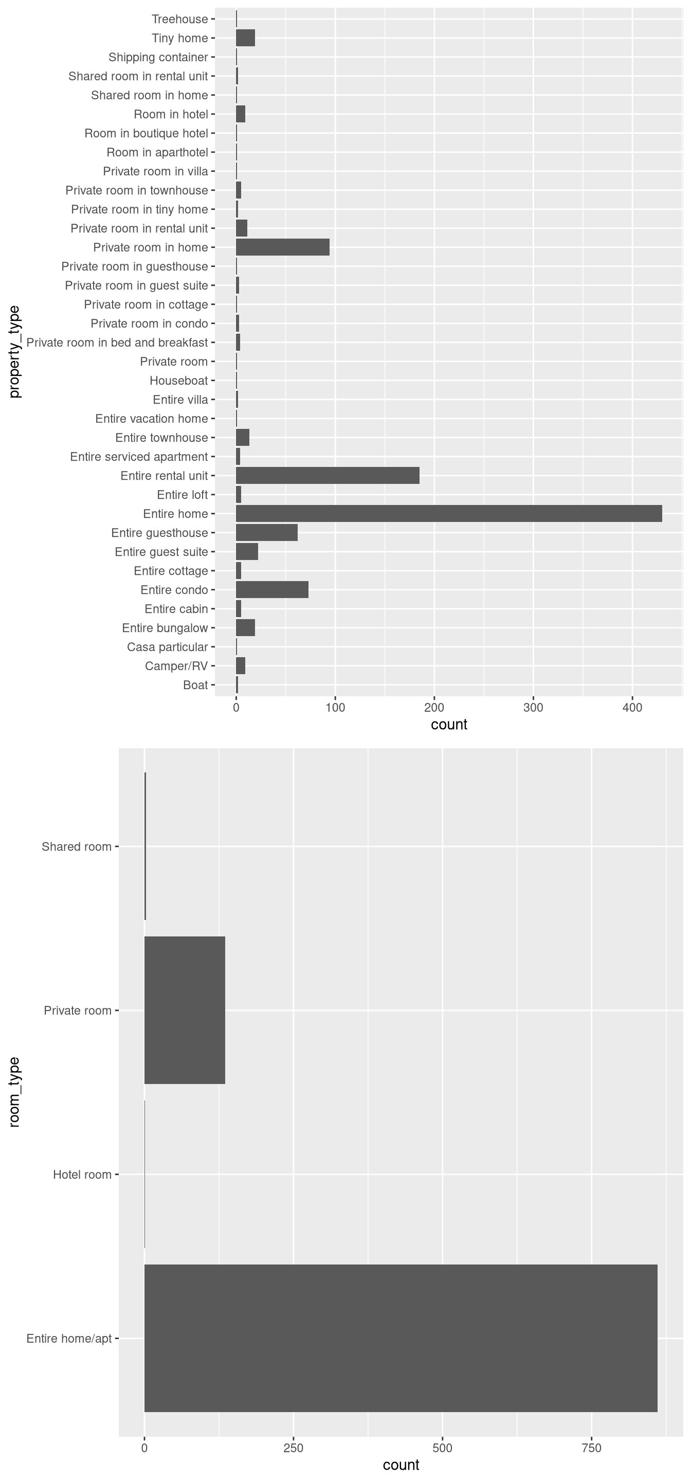

The property type graph shows a clear majority of listings are entire homes or rental units, which is unsurprising given Airbnb marketing. A notable thing I noticed here was that there were listings that were rooms in hotels, which seemed contradictory to the whole concept of Airbnb.

Variable relationship exploration

plot_correlation(austin_listings)

1 features with more than 20 categories ignored!
property_type: 36 categories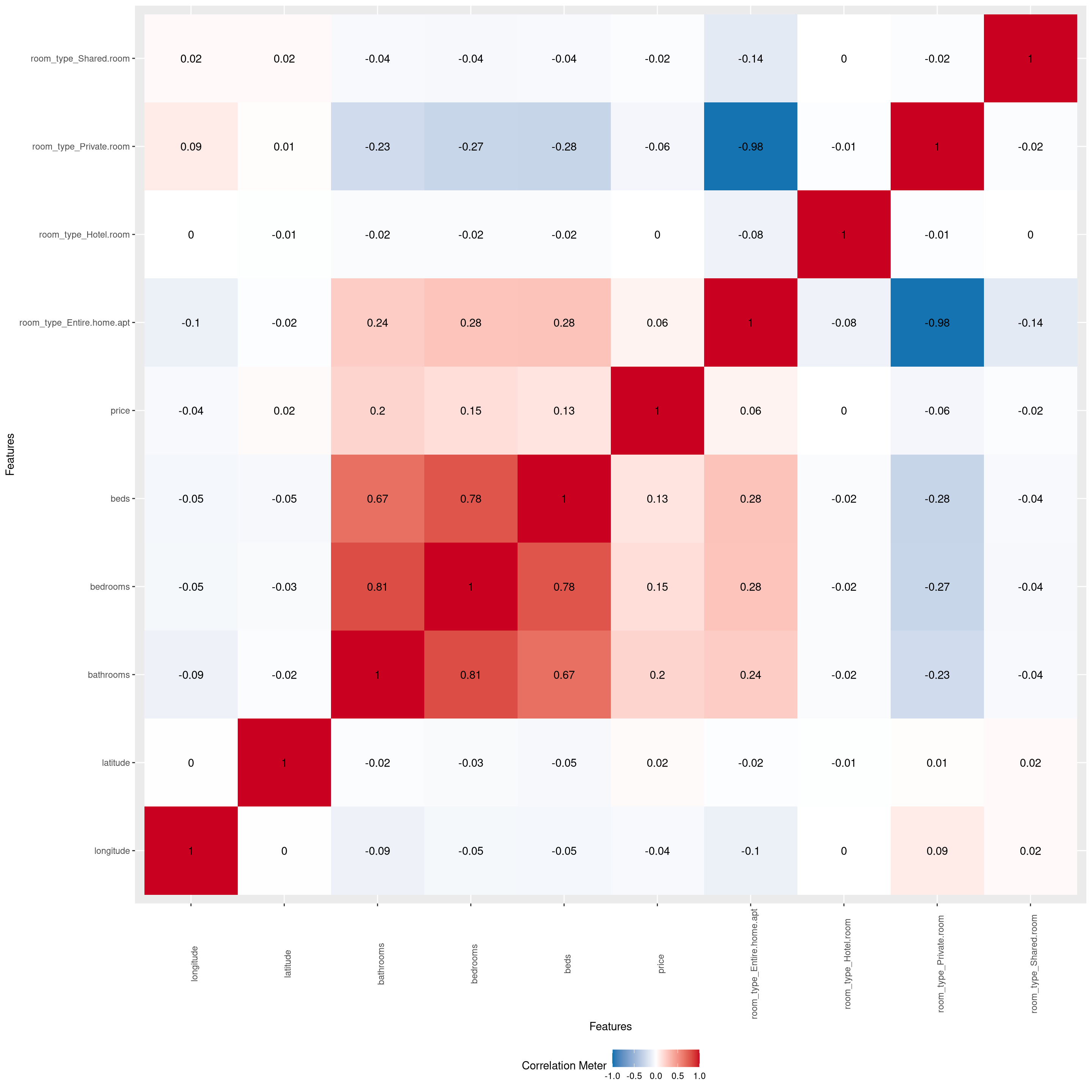

We can see some noticeable correlation among many of the predictors, with the private room type and the entire home apartment room type having the strongest correlation.

Now that we’ve gotten an understanding of what our data looks like, we proceed to the non-spatial analysis component.

Non-spatial analysis - LASSO regression for variable selection

library(glmnet)

Loading required package: Matrix


Attaching package: 'Matrix'

The following objects are masked from 'package:tidyr':

    expand, pack, unpack

Loaded glmnet 4.1-8

set.seed(0)

pred <- austin_listings %>% select(-price)
X <- data.matrix(pred)
y <- austin_listings$price

cv.model <- cv.glmnet(X, y, alpha = 1)
lam <- cv.model$lambda.min

best_mod <- glmnet(X, y, alpha = 1, lambda = lam)
coef(best_mod)

8 x 1 sparse Matrix of class "dgCMatrix"
                    s0
(Intercept)    46.0619
longitude       .     
latitude        .     
property_type   .     
room_type       .     
bathrooms     124.2221
bedrooms        .     
beds            .

Based on the LASSO method of variable selection, only the variable bathrooms is a significant predictor for the price of a individual listing. However, knowing there is another variable with relation to price helps us decide the specific kriging method for the best price prediction model.

With that, we move on to geospatial analysis.

Geospatial Analysis

h-scatterplots and correlogram

library(sp)
library(gstat)

sp_listings <- austin_listings

coordinates(sp_listings) <- ~ longitude + latitude

qq <- hscat(price ~ 1, sp_listings, c(0, 20, 40, 60, 80, 100, 120, 140, 160, 180))

plot(qq, main = "h-scatterplots")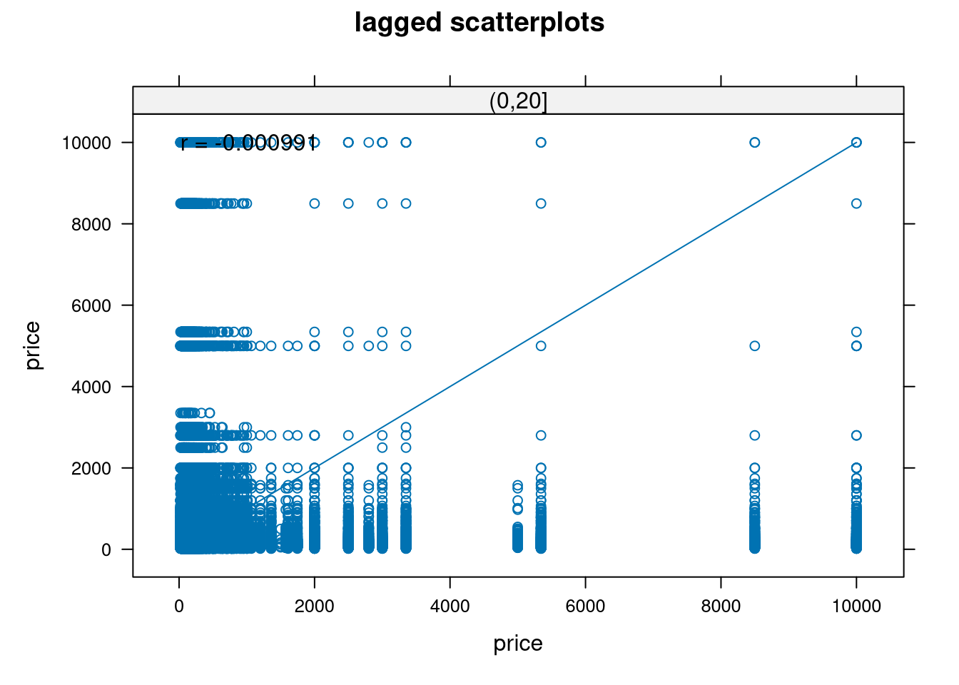

plot(c(10, 30, 50, 70, 90, 110, 130, 150, 170), c(0.824, 0.811, 0.734, 0.684, 0.629, 0.517, 0.473, 0.37, 0.264), type = "l", xlab = "Separation distance (h)", ylab = "Correlation coefficient (r)", main = "Correlogram for AirBnB pricing data", xaxt = "n", yaxt = "n")

axis(1, at = seq(10, 240, by = 20), labels = seq(10, 240, by = 20))

axis(2, at = seq(0, 1, by = 0.1), labels = seq(0, 1, by = 0.1))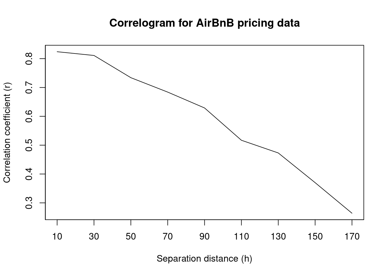

Both the h-scatterplots and the correlogram indicate that there seems to be spatial correlation between points. This is especially noticeable in the correlogram as we can visualize a clear negative trend in correlation coefficient as the separation distance increases. This seems to justify our spatial correlation approach.

Variograms

Sample variogram

Scaling is done here to make variogram creation easier later on.

g <- gstat(id = "scaled price", formula = scale(price) ~ 1, locations = ~ longitude + latitude, data = austin_listings)
samp <- variogram(g)
plot(samp)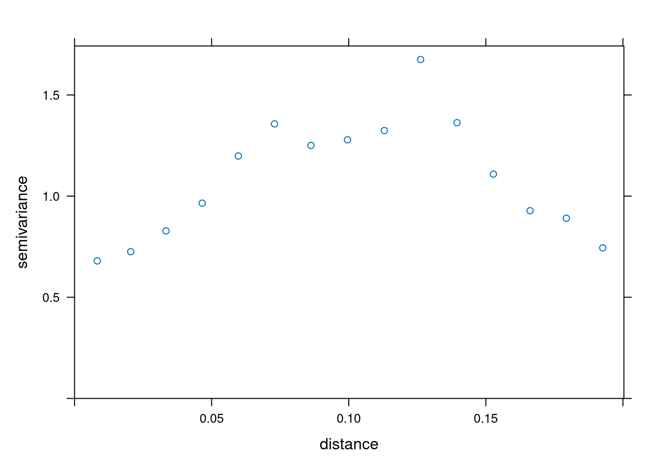

Different covariance function fits (using Cressie’s weights)

We use Cressie’s weights as a compromise between the techniques of ordinary least squares and generalized least squares. This way we can reduce computation but also account for covariance structures.

The two selected covariance functions are the exponential and spherical covariance functions.

exp_fit <- fit.variogram(samp, vgm(1.2, "Exp", 0.7, 0.3), fit.method = 2)
sph_fit <- fit.variogram(samp, vgm(1.2, "Sph", 0.7, 0.3), fit.method = 2)

plot(samp, exp_fit)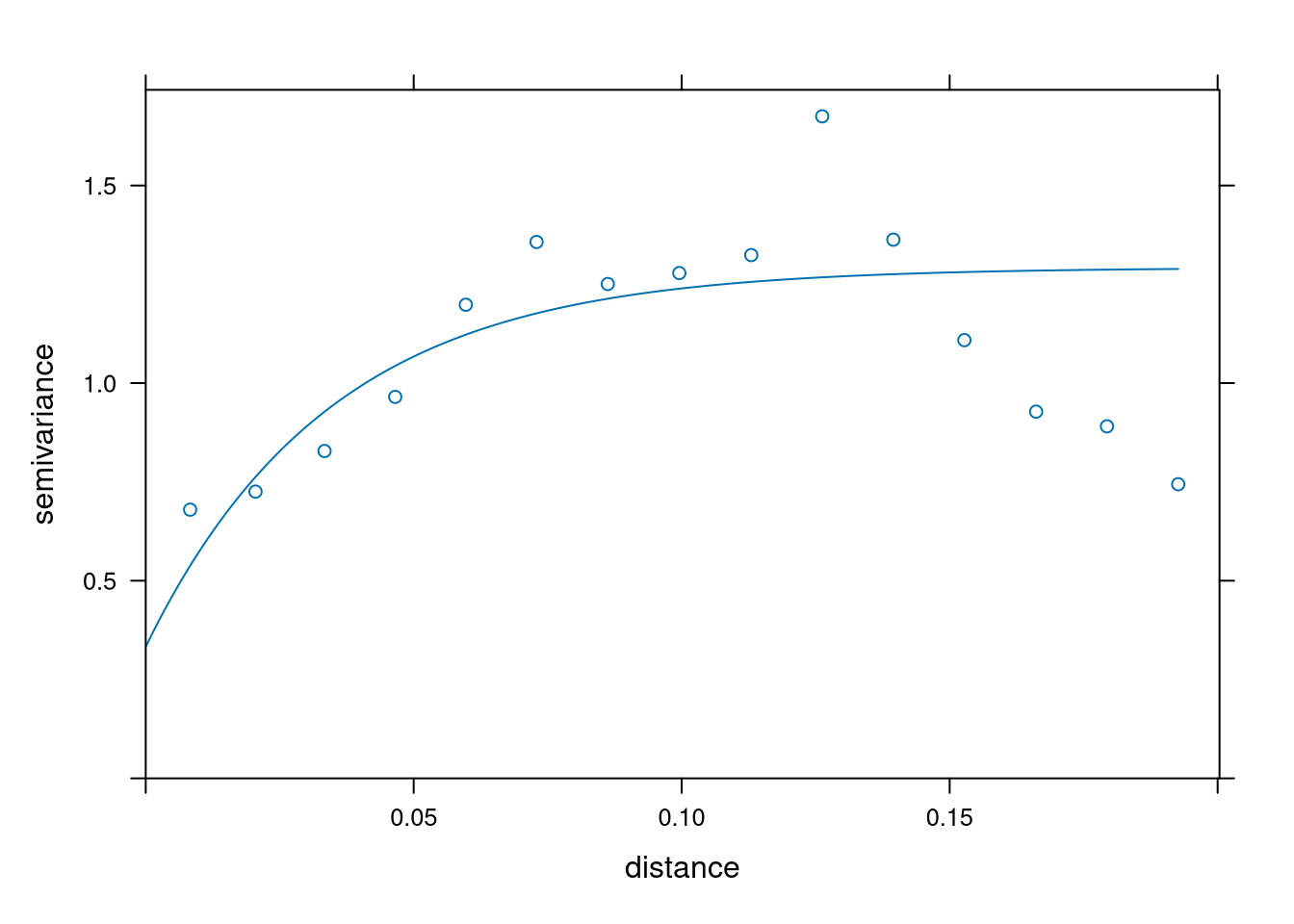

plot(samp, sph_fit)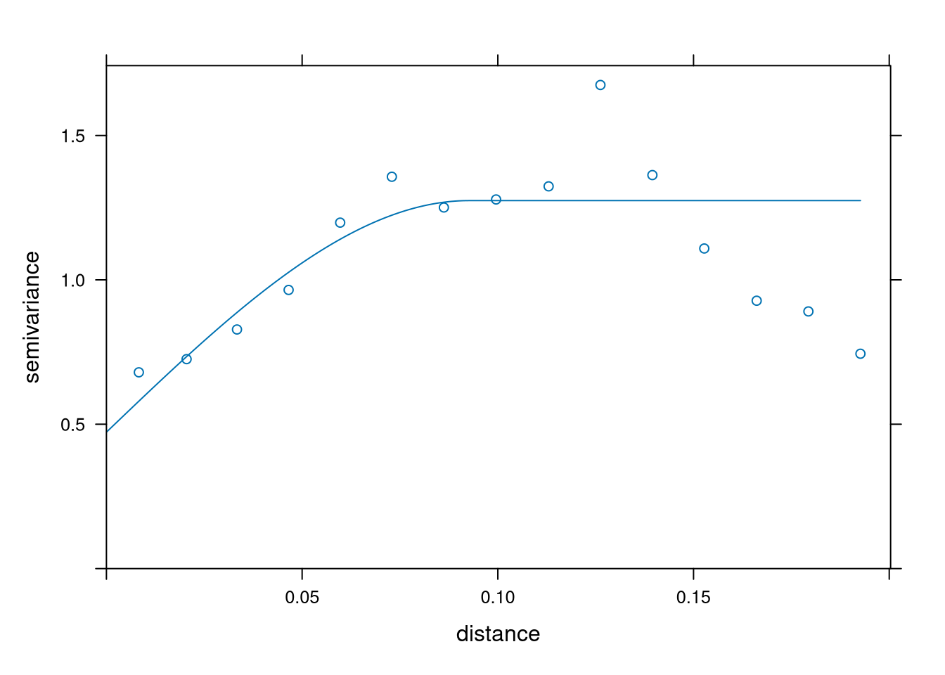

Visually it is hard to choose the best covariance function. Instead, we will minimize PRESS (predicted residual error sum of squares). Through cross-validation, we’ll select a covariance function for our model.

Cross validation

sl <- sample(1:1000, 700)

train <- austin_listings[sl, ]
test <- austin_listings[-sl, ]

cvalid <- krige(id = "scaledprice", scale(price) ~ 1, locations = ~ longitude + latitude, model = exp_fit, data = train, newdata = test)

[using ordinary kriging]

difference <- scale(test$price) - cvalid$scaledprice.pred
summary(difference)

       V1          
 Min.   :-2.88004  
 1st Qu.:-0.20605  
 Median :-0.10193  
 Mean   : 0.01401  
 3rd Qu.: 0.03235  
 Max.   :13.60095

press1 <- sum(difference^2)
press1

[1] 314.8996

cvalid <- krige(id = "scaledprice", scale(price) ~ 1, locations = ~ longitude + latitude, model = sph_fit, data = train, newdata = test)

[using ordinary kriging]

difference <- scale(test$price) - cvalid$scaledprice.pred
summary(difference)

       V1           
 Min.   :-1.941282  
 1st Qu.:-0.220706  
 Median :-0.125659  
 Mean   : 0.005639  
 3rd Qu.: 0.000283  
 Max.   :13.555199

press2 <- sum(difference^2)
press2

[1] 304.6792

We see here that the spherical covariance model minimizes PRESS so we continue onward with this covariance function.

Kriging

We know there is one related variable, bathrooms, that has the most correlation with price. Let’s investigate whether cokriging with this predictor would be the best approach to price prediction.

Ordinary kriging

x.range <- as.integer(range(austin_listings[, 1]))
y.range <- as.integer(range(austin_listings[, 2]))
grd <- expand.grid(
  longitude = seq(from = x.range[1], to = x.range[2], by = 0.001),
  latitude = seq(from = y.range[1], to = y.range[2], by = 0.001)
)

pred <- krige.cv(formula = scale(price) ~ 1, data = austin_listings, locations = ~ longitude + latitude)

mean(pred$residual)

[1] 0.01774772

Ordinary Co-kriging

Adding the covariate and looking at the variogram plots:

all <- gstat(g, id = "bathrooms", formula = scale(bathrooms) ~ 1, locations = ~ longitude + latitude, data = austin_listings)

var_all <- variogram(all)
all_fit <- fit.lmc(var_all, all, model = sph_fit)
plot(var_all, all_fit)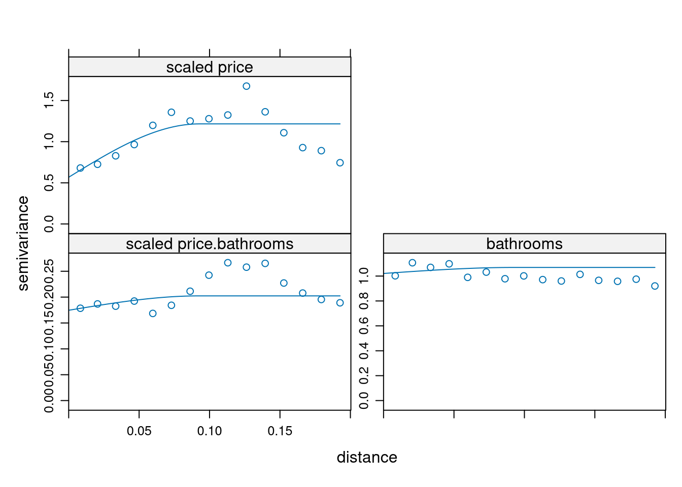

ck <- predict(all_fit, grd)

Linear Model of Coregionalization found. Good.
[using ordinary cokriging]

cok <- gstat.cv(all_fit)

Warning in checkNames(value): attempt to set invalid names: this may lead to
problems later on. See ?make.names

print(head(pred))

     var1.pred var1.var   observed    residual zscore fold longitude latitude
1  0.157460703       NA -0.1568927 -0.31435337     NA    1 -97.74668 30.27257
2  0.004633452       NA  0.2780841  0.27345065     NA    2 -97.72470 30.25387
3 -0.010727639       NA -0.2721183 -0.26139066     NA    3 -97.72851 30.24386
4 -0.105715907       NA -0.1266459 -0.02093003     NA    4 -97.74562 30.25795
5 -0.053681854       NA -0.1684152 -0.11473337     NA    5 -97.74712 30.27016
6  0.015238444       NA  0.2838454  0.26860694     NA    6 -97.72518 30.25520

print(head(ck))

  longitude latitude scaled price.pred scaled price.var bathrooms.pred
1   -98.000       30        0.03859578         1.242966       0.086515
2   -97.999       30        0.03859578         1.242966       0.086515
3   -97.998       30        0.03859578         1.242966       0.086515
4   -97.997       30        0.03859578         1.242966       0.086515
5   -97.996       30        0.03859578         1.242966       0.086515
6   -97.995       30        0.03859578         1.242966       0.086515
  bathrooms.var cov.scaled price.bathrooms
1      1.073499                  0.2039032
2      1.073499                  0.2039032
3      1.073499                  0.2039032
4      1.073499                  0.2039032
5      1.073499                  0.2039032
6      1.073499                  0.2039032

library(lattice)

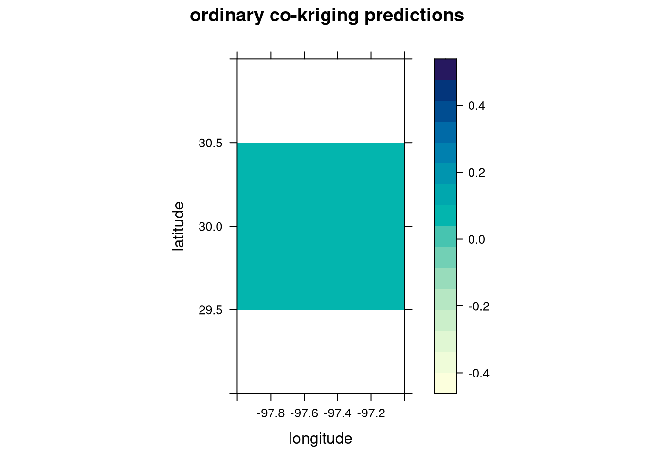
levelplot(ck$`scaled price.pred` ~ longitude + latitude, ck,
  aspect = "iso",
  main = "ordinary co-kriging predictions"
)

levelplot(ck$`scaled price.var` ~ longitude + latitude, ck,
  aspect = "iso",
  main = "ordinary co-kriging variance"
)

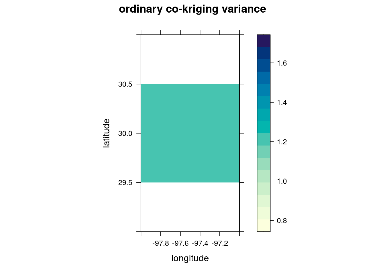
We can see lots of uniformity between the co-kriging predictions and variance. Is it better than ordinary kriging?

In this case, it looks like ordinary kriging is better as the cokriging results are too uniform and don’t accurately capture the variation in pricing amongst Austin listings. Therefore, our final model is the spherical covariance model with ordinary kriging.

Note for ultimate Kriging Predictions

It should be noted that for the purposes of actual price prediction, the inputs of this model must be scaled which means that the resulting predictions have to be un-scaled to the original units.